Logistic Regression

Logistic regression algorithm finds a linear function that predict class ($\hat{y}$) given an input vector $x$ as,

\begin{equation} \hat{y}=\sum_{n_x}^{j=0} w_jx_j+b=w^Tx+b \end{equation}

The final goal here is to find optimal weights $w$ that best approximate the output y by minimizing the prediction error. The simple loss function or error function is one half of square error as, \begin{equation} L(\hat{y},y)=\dfrac{1}{2}(\hat{y}-y)^2\approx 0 \end{equation}

Typicaly, the output should be in probability form ($0<\hat{y} <1$), and thefore sigmoid function ( or similar function) is applied to predicted output. So that the final Logistic regression can be shown by, \begin{equation} \hat{y}=P(y=1|x) \longrightarrow \hat{y}=\sigma(w^Tx+b) \end{equation}

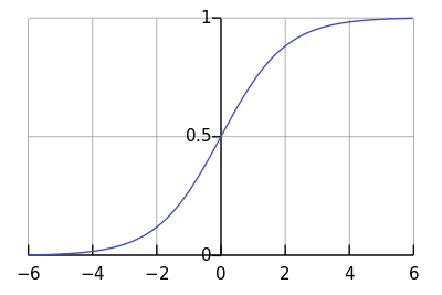
The sigmoid function, $\sigma(z)= \dfrac{1}{1-e^-z}$, gives an $S$ shaped curve as shown in Figure 1. $\sigma(z)= 0$ when $z\longrightarrow -\infty$ and $\sigma(z)= 1$ when $z\longrightarrow +\infty$. The $\sigma(z)=0.5$ when $z=0$. Therfore, If the output is more than $ 0.5 $, the outcome can be classify as 1 and 0 otherwise.

The half a square error might cause the optimization problem (non-convex problem). To prevent multiple local optima the loss function can be written as,

\begin{equation} L(\hat{y},y)=-\big(y\log \hat{y}+(1-y)\log(1-\hat{y}) \big) \label{eq:loss} \end{equation}

Above equation measures how well th model is for one a single training example. The overall performance over $m$ training is indicated by cost function $ J $ as,
\begin{equation} J(w,b)=\dfrac{1}{m} \sum_{i=1}^{m} L(\hat{y}^i,y^i) \label{eq:cost} \end{equation}